
Part VII: The survival of the plessists
VII.1.0 If you have not read the relevant section, then please go here for a definition of ‘plessists’.
VII.1.1 We began our journey by highlighting biology and ecology’s abject failure to provide adequate definitions for their core concepts. We shall conclude that journey by proving that a population free from Darwinian fitness, competition, and evolution is simply impossible.
VII.1.2 Nothing makes the parlous state of affairs in the biological sciences clearer than the definition for natural selection—the acknowledged centrepiece of all theoretical and experimental biology—offered by the Collins Dictionary of Biology:
natural selection, n. the mechanism, proposed by Charles Darwin, by which gradual evolutionary change takes place. Organisms which are better adapted to the environment in which they live produce more viable young, so increasing their proportion in the population and thus being ‘selected’. Such a mechanism depends on the variability of individuals within the population. Such variability arises through mutation, the beneficial mutants being preserved by natural selection (Hale & Margham, 1988).
This neatly exemplifies the vagueness, the circularity, and the lack of rigour that bedevils these subjects. Anyone wanting further clarity about natural selection—the sine qua non of all modern biology—is referred straight back to the same head word!
VII.1.3 Our own work has already provided a complete contrast to the above-described state of affairs. We have already framed a comprehensive collection of laws, maxims, and constraints, and provided clarity and some clear definitions for core concepts. We did so by dint of turning to topology and observing that reproduction is homeomorphic with the two embedded processes of (a) sets, and (b) self-replications which were first demonstrated, in the coordinated ways we require, by the German mathematicians Karl Weierstrass and Georg Cantor. They allow us to unambiguously quantify natural selection.
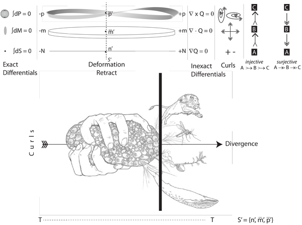
VII.1.4 We take τ as the given generation length, and N as the mean number across whatever given interval. We can then quantify every population’s changes in its numbers as its numeracy, Q, where both Q = dN⁄dt and N = ∫Q dt for absolute clock times; and N = ∫Q dτ and Q = dN⁄dτ all across the circulation. We can also relate all changes to each other as a set of inexact differentials that match the exact differential ∫dS = ∫dN = 0. Those inexact differentials in numeracy are:
• ∇Q = (nfinal - ninitial)⁄N as the gradient;
• ∇ • Q = m̅final - (m̅initialninitial ⁄nfinal) as the divergence;
• ∇ × Q = p̅finalm̅initial(nfinal - ninitial) as the curl.
Natural selection is then the combination of those exact and inexact changes in numeracy over each of (i) the absolute time, T; (ii) the circulation length, τ; and (iii) the transition between minimum and maximum values.
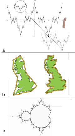
VII.2.1 The first ingredient we need to prove that a population free from Darwinian fitness, competition, and evolution is impossible is the first ever “self-replicating curve”, seen in Figure 42a. Created by Weierstrass, it serves as a successful and explicit mathematical model for biological replications because it is (A) “everywhere smooth”, and (B) “nowhere differentiable”. This simply means that it has a topology that has no holes anywhere, while its complexity, in the sense of its curvaceousness, also varies in regular and repetitive fashion.
VII.2.2 We imagine catching hold of Weierstrass’ curve, and pushing or pulling it along its axis, and as shown in Figure 42a. Since it is everywhere smooth, then it is always continuous. It can keep projecting itself, all along its length, indefinitely and infinitely in its given directions—which is in our case both into the past and into the future. And since it is a repeating curve, then we can easily select a final moment t1; an initial moment t-1; and determine its rate of propagation across that interval, which is the distance it covers per unit time, dτ⁄dt. But since the curve must cover some specified distance along its length, that actual distance is ∫ τ dt, and is clearly subject to variation as the curve proceeds.
Since the curve is non-linear, then any population following it must undertake a set of accelerations both along that curve and between the moments t-1 and t1. That change in the rates of propagation, at any given point, is d2τ⁄dt2. The distance covered in undertaking all such changes, across the same interval—and which is also subject to variation—is ∬τ dt dt.
And, finally, if the population is to cover both sides of Boy’s surface; and/or traverse both of the biology and replication globes; and/or return to the Möbius strip contact point; then it must undertake the relevant series of jerks, between t-1 and t1, and as d3τ⁄dt3. That total distance about both globes is ∭τ dt dt dt.
Every self-replicating curve—and therefore every viable population—will have these seven values at each specified moment t0 between t-1 and t1. They use the standard rectilinear ijk axes of absolute measures and absolute time. We can place this initial set of seven absolute time-based values in a first set, P.
VII.2.3 We can next measure the self-replicating curve’s complexity. This is its amplitudinal rapidity in propagation. It reflects the amount of self-replication that passes by at each moment. We can do so through the nowhere differentiable aspect of Weierstrass’ curve. Nowhere differentiable means that no matter how closely we approach the curve to determine its rate of change, we always find a complete and entire copy of the original. Weierstrass’s entire curve can replicate itself between any two points and/or moments. This embedded self-replication also continues indefinitely. This change in what is replicated at each point and moment is a second rate of propagation that accompanies the first.
VII.2.4 Working independently of Weierstrass, the English mathematician, physicist, meteorologist and psychologist Lewis Fry Richardson further developed these ideas on rates of replications and self-replications. Figure 42b’s “Richardson effect” is the latter’s observation, as applied to Great Britain’s coast line, that the smaller we make our ruler, and so the finer our subdivisions become, then the greater is the number of bays and inlets we can measure around, and so the longer becomes the perimeter. This is a varying rate of propagation.
VII.2.5 If all our perimeter points now form a first set A; and if all the points constituting the area form a second set B; then the one-dimensional measure in A tends to infinity, at some given and measurable rate, even as the two-dimensional measure in B remains invariant. But since, no matter what the scale, we recreate the entire area at some rate every time we go all about the perimeter, then the rate at which the replication occurs about the perimeter, and so the rate at which we bound and traverse an area, depends upon the rate at which we scale the perimeter.
VII.2.6 When the Polish-born mathematician Benoit Mandelbrot was clearing out some of Richardson’s old papers, he came across the Richardson coastline paradox. He developed and popularized the ideas behind these embedded self-replications (Hunt 1998). He produced his famous fractals.
A self-replicating fractal’s “dimension”, D, states the number of self-similar replicas we can find, N, as the scaling factor, ε, changes. It is given by D = -logN/logε.
If we first take up a Euclidean straight line, then its fractal dimension means that no matter how often we scale and replicate it, it always remains equal to the space it resides in. If we decompose it into four segments, a magnification factor of ε = 4, we get four line segments, all self-similar. If we magnify each of those by 4, we recover the original. So if, more generally, we decompose it N times over, we will find N self-similar copies that again restore the original. A Euclidean straight line segment therefore has the fractal dimension D = 1. This means that the curve’s current rate of propagation is equivalent to that of a Euclidean line. It indicates the degree of complexity—or, alternatively, the number of events—involved in any given self-replication. These are in this case the same. The number of points in any set may in principle be uncountable, but its fractal dimension will still tell us how self-similar it is as it replicates.
A square, in the Euclidean plane, behaves somewhat differently. If we use the same ε = 4 magnification factor, we end up with a square that is 1⁄4 × 1⁄4 = 1⁄16th times the size. We will now need 16 self-similar squares to recover the original. So for any N, we will always have N2 self-similar pieces. The square therefore has the fractal dimension D = 2.
On this same basis, the fractal dimension of a cube is D = 3, and that of a tesseract (four-dimensional hypercube) is D = 4. Every four-dimensional object is now “bigger” than every three-dimensional one, which is in its turn bigger than any object in the plane, which is bigger than one on a line, with each having a successively smaller fractal dimension … meaning that each self-replicates at an equivalently greater rate. So if we consider two or three manifolds or dimensions, and they all behave in Euclidean fashion, then they will deliver the appropriate fractal dimensions.
All self-similar one-dimensional objects are also curves in the plane. They therefore have a fractal dimension lying between 1 and 2. So if, for example, Great Britain’s coastline quadruples in length every time we use a ruler 1/3 the size, then we have ε = 3 and N = 4, giving it a fractal dimension of D = -logN/logε = 1.2619. The complexity of Britain’s coast line—the way in which it changes as we approach it ever more closely—therefore lies somewhere between that of a line and a plane.
Although no three-dimensional “Mandelbrot set” can be built in that there is no three-dimensional analogue for the field of complex numbers, the principle still holds for two and three dimensions. Just as a one-dimensional manifold, such as a coastline, exhibits its changes in complexity upon a plane, so do two dimensions exhibit theirs in a three-dimensional realm. The complexity or fractal dimension for any two-dimensional object we create by bringing two distinct dimensions together lies between 2 and 3. And, similarly, a three-dimensional object exhibits its complexities and self-replications with some value between 3 and 4.
Every self-replicating curve will replicate its curves, its shapes, and its complexities at some rate, over any interval, that in its turn depends upon its development at each specified point. But we can always express this self-replication rate in terms of the rate it maintains between its initial and its terminal values. If we express the average complexity across the curve as D’, then the value at each point is some rate that is a function of D’ and is given by d = D/D’. Its various derivatives and integrals will be dd/dD’ and ∫ d dD’; d2d/dD’2 and ∬d dD’ dD’; and d3d/dD’3 and ∭d dD’ dD’ dD’. These tell us the changes in complexity relative to each other, and as they influence each other in a cycle. The complexity transitions use a mean that repeats, and that also states each succeeding value in terms of a prior one, thus ultimately completing a circulation about that mean. These additional seven measures use Newton’s hyperspherical IJK axes. We can place them in a second set, Q.
VII.2.7 Every self-replicating curve has both (a) a perimeter length, τ; and (b) a fractal dimension, D. These do not all develop in the same ways relative to each other, as the curve propagates in time, t. Since every population travels along its curve as if it is a one-manifold that is a Euclidean straight line, then each will have a different rate of self-replication per unit of its length, due to its different shape and non-differentiable component. If we express the value at each point as s = D/τ, then the rate is ds/dτ. The amount replicated across any interval is always ∫ s dτ. And since the greater is the complexity, then the greater must be the acceleration through those changes, then we also have d2s/dτ2 and ∬s dτ dτ; and we have d3s/dτ3 and ∭s dτ dτ dτ to traverse the Möbius strip. This final set of seven measures links a curve’s diversity in its complexity directly to its own length, and to its own amplitudes or changes on its own length, and uses the Frenet-Serrat frame’s TNB axes. We can place them in a third set, R.
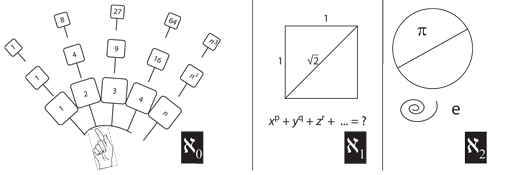
VII.3.1 The next ingredient we need to prove that a population free from Darwinian fitness, competition, and evolution is impossible is the “paradox of the infinite series of square numbers”, shown in Figure 43. Although the paradox was known long before Galileo, since it received a particularly famous retelling in his epoch-making Discourses and Mathematical Demonstrations Relating to Two New Sciences, it is frequently named after him.
The Galileo paradox points out that while the ordinary counting numbers form the infinite series 1, 2, 3, 4, …, n, …, their squares form the very different—but equally infinite—series 1, 4, 9, 16, …, n2, …. This gives the distinct impression, for the paradox’s first part, that the “density of the squares”, amongst the natural numbers, is considerably less than is the density of the ordinary natural numbers. This density effect is even more pronounced amongst the cubes, which go 1, 8, 27, 64, …, n3, …. The perceived gaps grow even more quickly.
VII.3.2 Galileo also pointed out, for the paradox’s second part, that this initial impression must be false. We will never run out of numbers. Since we will never fail to find an n2 or an n3 to accompany any n, then the densities must be equal. So in spite of the initial impression, the squares and cubes must be equinumerous with the ordinary natural numbers. But … these cannot both be true.
VII.3.3 The German mathematician Georg Cantor resolved the Galileo paradox by pointing out that we can place all possible natural numbers in a single set. He denoted it ℵ0. Since all squares, all cubes, and all possible rational numbers—such as 133/139ths—come from that same set, then they are all equipollent with the countably infinite natural numbers (Weisstein 2015a).
VII.3.4 Cantor next pointed out that the ℵ0 set is deficient because no possible combination amongst them can produce the “irrational numbers” that we need to solve even the simplest of purely algebraic equations such as the a2 + b2 = c2 of the Pythagoras theorem and which tells us that the length of a square’s diagonal is √2. Since that √2 is nowhere in ℵ0, then we must create a second infinite set to solve all such algebraic equations. And since this new set can contain all the infinitely many numbers in the first set, ℵ0, then that ℵ0 is injective, ![]() , into ℵ1. But further since ℵ1 contains infinitely many more numbers than can be contained in ℵ0, then ℵ1 is in its turn surjective,
, into ℵ1. But further since ℵ1 contains infinitely many more numbers than can be contained in ℵ0, then ℵ1 is in its turn surjective, ![]() , over ℵ0.
, over ℵ0.
VII.3.5 But that was not the end of Cantor’s demonstrations. Neither π nor e, he pointed out, is the solution to any algebraic equation. There is in fact a whole host of numbers that are not algebraic for they are not the roots of non-zero polynomial equations with rational coefficients. There must, therefore, be a yet larger set of numbers containing those yet even infinitely many more “transcendental numbers”. He designated that latest set ℵ2.
VII.3.6 Since both the previous ℵ0 and ℵ1 sets are smaller than this newest one, then they are both injective into this latest ℵ2, which is in its turn surjective over both those ℵ1 irrationals and ℵ0 rationals.
VII.3.7 We also notice very carefully that we can draw conclusions about the interactions between these various sets based on their relative sizes, and so on their injections, surjections, and possible bijections, and all without determining any specific numbers contained in each. The same goes for the fractal dimensions and their measures of replication and self-replication through the ijk, IJK, and TNB axes.
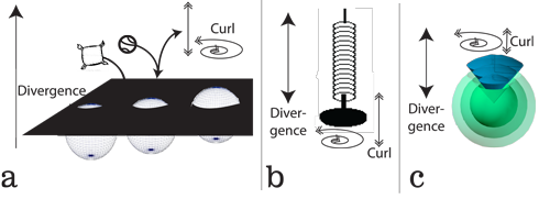
VII.4.1 We need one further ingredient to complete our proof. The French mathematician Baron Augustin-Louis Cauchy showed how we can analyse the various situations we see in Figure 44, which all involve various kinds of transformations.
Whether a ball bounces, a cushion merely falls, or we pass a three-dimensional (x, y, z) rotahedron in the z-direction through a two-dimensional (x, y) surface, we need to assess all possible shapes and transformations, and their rates of change, across all those various dimensions. We can do so using Table 1’s “Cauchy tensor”:
Table 1
The Cauchy tensor
| x (length) |
y (breadth) |
z (height) |
|
|---|---|---|---|
| x (length) | xx | xy | xz |
| y (breadth) | yx | yy | yz |
| z (height) | zx | zy | zz |
If we push a rotahedron through the plane, in the z direction, then the zx term tells us how much of that z push has been deformed and flattened into x as the rotahedron has changed its shape, and has splurged out into that lateral dimension instead of proceeding vertically to the required degree. The zy similarly tells us how much it might have deformed into y with that same push.
However, it also works the other way. We can carefully measure a circle in the x and y dimensions as (x1, y1), and (x2, y2). We can then calculate a Cauchy tensor xz component to express the force the circle exerted, as an inexact differential, that was originally into the x direction, but that must have diverted into z. The same again goes for yz.
The spring in Figure 44b shows that we can indeed determine the overall forces, both exact and inexact, falling upon, and exerted by, any object and its materials. We simply analyse all its forces and effects in each selected direction.
The xx, yy, and zz components located along the Cauchy tensor’s diagonals are the “normal pressures” that reveal an object’s most characteristic responses. They are each object’s attempt to hold its shape, whether it be a cushion, a spring, a rotahedron, a bouncing ball, or a self-replicating curve. All an object’s off-diagonal components are then its “shear stresses”. They summarize the overall distortions imposed by the surroundings, and/or that are caused by its material’s deformities.
We can just as easily construct a Cauchy tensor by putting a self-replicating curve’s length, τ, fractal dimension, D, and dimension per unit length, s, as the heads of the rows and columns to create each component.
VII.4.2 The normal forces in any Cauchy tensor are also our divergences. We can always determine them by determining the average transformation, and the average distances, in each given direction. The divergence is then always whatever constant rate of change occurs in alignment with whatever given direction, and to and over both time and space. Thus a self-replicating curve can have a divergence in its length; in its fractal dimension; and/or in its dimensionality per unit length. A zero divergence always means the amounts entering and leaving are the same.
The shear forces in any Cauchy tensor are then the curls. They are (a) the variations about whatever average creates the divergence; and/or (b) the transformations that any divergence causes in some other direction. These all apply just as well to the sphere in Figure 44c. Since time is one of our directions, then a curl can be any variation over time, such as a velocity, acceleration, or jerk, all of which are with respect to t; or else a partial differential of the form ∂x⁄∂t. If divergences are constant then there is no curl; and if there is a curl then there must be a change in divergence somewhere.
VII.4.3 We should also recollect that our biological entities—our plessists and our plessemorphs—follow all rules for sets. So any two sets of plessists X and Y can always be associated via their Cartesian product X × Y which forms all possible duples (x, y) where x is in X, and y is in Y. And similarly, X, Y, and Z can form X × Y × Z = {(x, y, z) | x ∈ X, y ∈ Y, z ∈ Z}.
VII.4.4 The three sets P, Q and R that we form from our self-replicating curves also follow Cartesian product rules. As in Table 2, we can therefore use their 21 elements to form a single component in a Cauchy tensor. Table 1’s 3 × 3 Cauchy tensor with its 9 components would therefore be constituted of 21 × 9 = 189 such elements, each one contributing to the whole.
Each individual component in our self-replicating curve’s Cauchy tensor has the structure:
Table 2
The 21 elements in a single Cauchy tensor component
|
3rd derivative |
2nd derivative |
1st derivative |
value |
1st integral |
2nd |
3rd |
||
|
absolute time, |
← ijk |
d3τ⁄dt3 |
d2τ⁄dt2 |
dτ⁄dt |
τ |
∫τ dt |
∬τ dt dt |
∭τ dt dt dt |
|
min–max |
↑ IJK |
d3d⁄dD’3 |
d2d⁄dD’2 |
dd⁄dD’ |
d |
∫d dD’ |
∬d dD’dD’ |
∭d dD’ dD’ dD’ |
|
relative time, |
■ TNB |
d3s⁄dτ3 |
d2s⁄dτ2 |
ds⁄dτ |
s |
∫s dτ |
∬s dτ dτ |
∭s dτ dτ dτ |
Any observed value is a combination of: (i) the homotopic and homotopically equivalent τ; (ii) the homeomorphic replication inherent in each point in the circulation as d; and (iii) the isomorphic state for that specified group of transformations—as can create a species—as s.
Both (a) the overall quantities, and (b) the rates of change in each of the three forms of the changes we discovered, as τ, d, and s, are determined by their coordinated juxtapositions in their integrals and derivatives, and all over 0, 1, 2 and 3 dimensions. These and their fractal dimensions then ensure that the entities remain neighbours all about the given circulation. If they are biological entities then they define the same base, B, between the progenitor domain as preimage, X, and progeny codomain as image, Y, by sharing all rates, quantities, and distances That base is formed from:
BXY = {U(X) × V(Y) | U open in X, V open in Y},
and
BYX = {U(Y) × V(X) | U open in Y, V open in X},
and so that B = BXY ∪ BYX, with the intersection of BXY ∩ BYX being constantly nonempty.
VII.4.5 Our base is now a mixture of three different kinds of self-replications. We can measure them through their fractal components, using the three different kinds of axes we have discovered:
• ijk. The top row of 21 elements making up each distinct tensor component ensures that its interactions with the universal covering space, C, and mapping cylinder, Mλ, that are the surroundings are constantly homomorphic and homotopically equivalent. This top row of elements in each component contributes to the set of absolute and real time rectilinear ijk axes in ordinary space and time. Its transformations are exerted in, and are presented to, the surroudings. It is the surface forces, S. They emerge as a form of momentum. Each top row thus helps determine the temporal value through its horizontal row in its Cauchy tensor.
• IJK. The middle row of 21 elements in each distinct tensor component establishes the homeomorphic paths that link each one successively to the next, all about a circulation. These values link every x to its dx, and so to the x at x-1 and x1. It therefore ranges from a minimum to a maximum around some x’ mean. These are the successive and therefore hereditary values transmitted from point to point, all about the circulation, and so across the generation. They together manifest as a form of contained energy, and energy density, within a given volume, V. Each middle row helps determine the values and succession of values in its Cauchy tensor’s vertical column.
• TNB. The bottom row of 21 elements in each distinct tensor component imposes the conditions for the prevailing isomorphisms. It determines the distinctive Sn-1–Vn-1,
Sn-1–Vn, Sn–Vn, Sn–Vn+1, and Sn+1–Vn+1 contributions that mesh all rows and columns. Each thereby coordinates with all its lower- and higher-level transformations as base, fibre, fibre bundle, helicoid, rotachoron, Möbius strip, and real projective plane. Each bottom row establishes the values and behaviours for that given component, and at that nexus of row and column.
VII.4.6 Now we know that we must have three different kinds of sets, and the three different kinds of ijk, IJK, and TNB axes which are of different sizes, we are ready to prove that a population free from Darwinian fitness, competition, and evolution is impossible.
VII.5.1 A topologically based investigation has the advantage of being extremely general. A topologist can, for example, deform a square into a circle in a way that is geometrically impossible, but still draw valid conclusions. In the same way, while an ant as large as a whale and a whale as small as an ant are both biologically impossible, we are free to investigate the general deformations and transformations available to them. An ant as our first species S1 = {n1, m̅1, p̅1} might not, in reality, be able to scale upwards to either of S1 = {φ1n1, φ1m̅1, φ1p̅1} or S1 = φ1{n1, m̅1, p̅1}, while a whale, as a second species S2 = {n2, m̅2, p̅2} might not be able to scale downwards to either S2 = {φ2n2, φ2m̅2, φ2p̅2} or S2 = φ2{n2, m̅2, p̅2}, but these are clearly two different kinds of transformations. Just as a topologist insists that a sphere is sufficiently different from a torus to force, for example, ‘genus’, g, to the heart of the subject, then so also is it possible that, quite irrespective of any particular species, the position of any φ is significant.
The S = {φn, φm̅, φp̅} proposal suggests that all three variables can scale with identical rates of change. The S = φ{n, m̅, p̅} proposal insists that all three share one in common. These are not, however, the same.
If φ{n, m̅, p̅} = {φn, φm̅, φp̅} then S = {φn, m̅, p̅} … which is in fact impossible. The only possibility, over all biological entities, is S = α{φn, κm̅, χp̅}, with a specific relationship holding between α, φ, κ, and χ, and so that neither α nor φ can scale any population without immediately also changing and scaling κ and χ … which are then a set of Darwinian variations. The scaling factors φ, κ, and χ are unique to each species, and are their rates of change of n, m̅, and p̅, respectively.
VII.5.2 The proposition that S = φ{n, m̅, p̅} = {φn, m̅, p̅} is, by contrast, the proposition that biological populations can only undertake the “affine transformations” that use φ as their sole scaling factor. It means that S’ = {n’, m̅’, p̅’} is invariant over all circulations of the generations. It insists that m and p are Euclidean, with the fractal dimension D = 1. We can now show that this is impossible.
VII.5.3 Memes 4 to 9 proposed a set of plessists and plessemorphs that communicate with the material world through ψ and γ as Ingredients 3 and 4 of molecules and photons. They and their biological-ecological processes, λ, are a first set, A. We can replace our plessists in A at any time t, at any point τ, and so over any stretch dτ–dt, with plessemorphs that have the identical effect, and so that naaa = n1a1. Since they form a one-manifold, they each have a fractal dimension between 1 and 2.
The plessists and plessemorphs in A construct their genes and genomes with molecules. These are the γ plessiomes counted as b1 in B. We can, on the same basis, substitute ba plesseomes, also in B, to produce the identical effect, so that na{ba} = n1{b1}. All collections of plessiomes and plesseomes and one-manifolds and so also have a fractal dimension between 1 and 2.
And our plessists and plessemorphs interact both with each other and with their surroundings using their plemes and plessetopes. These are their photons, ψ, as c1 and ca in C. The ca plessetopes can again substitute for the c1 plemes, so that n1{c1} = na{ca}. These, also, are a one-manifold with a fractal dimension between 1 and 2.
VII.5.4 Since each distinct entity is an a in A while its molecules are b in B; and since each a is composed of numerous molecules whose numbers can change while the entity count remains the same; then A is injective into B, with B being surjective over A. And when these two sets associate, they form the standard Cartesian product (A × B)C. We can also always isolate the distinct ABC and BAC from (A × B)C. The product formed from A and B has a fractal dimension lying between 2 and 3.
VII.5.5 And then since each molecule is a b in some set B; and again since each can have numerous energy levels and form a variety of chemical bonds while the molecular count remains ever the same; then B is injective into C, while C is surjective over B. They form the Cartesian product (B × C)A. We can isolate BAC and CAB. The product has a fractal dimension between 2 and 3.
VII.5.6 And finally, since each distinct entity is an a in A while its photons are c in C with each a therefore being composed of numerous photons whose numbers must change, by the second law of thermodynamics, but while the entity count can remain the same; then A is injective into C, with C being surjective over A. And when these two sets associate, they form the standard Cartesian product (A × C)B. We can also always isolate the distinct ABC and CAB. The product has a fractal dimension formed from A and C, and lying between 2 and 3.
VII.5.7 And then further since A is injective into B while B is injective into C, then A is injective into C, while C is surjective over B, which is surjective over A, so that C is also surjective over A. And whenever B injects into C, so also does some specified and determinable biological entity exist as some a in A. We never have A injecting into B, or B being surjective over A, without some c in C; we never have A injecting into C, or C being surjective over A, without some b in B; and we never have B injecting into C, or C being surjective over B, without some a in A. The true meaning of there always being a base B = BXY ∪ BYX, with BXY ∩ BYX being non-empty is that we at all times have the Cartesian product (A × B × C), so that both n1(a1, b1, c1) and na(aa, ba, ca) always exist as plessists and plessemorphs respectively. The resulting fractal dimension is always between 3 and 4
VII.5.8 Given that (A × B × C) always exists, then we can always find the various homeomorphic, path-preserving, and isomorphic mappings φ:A ↔ B, φ:A ↔ C, and φ:B ↔ C, with all such transformations exhibiting both some absolute time interval, T, and some circulation distance, τ.
VII.5.9 The elements c in C, as our plemes and plessetopes, are free to replicate and self-replicate using any method desired. The individual elements a in A and b in B over which they are surjective will simultaneously undertake the set of energy transformations ±dψ, ±d2ψ, and ±d3ψ so they increase from some initial level towards a maximum; down to some minimum; and then returning to their initial level; so that they form a nontrivial loop upon a real projective plane. There therefore exists a base in ψ that is surjective over A and B, and whose absolute time span is TP while its circulation distance is τp = 1.
VII.5.10 The elements b in B, as our plessiomes and plesseomes, are also free to replicate and self-replicate using any method desired. The individual elements a in A and c in C, they being surjective over the former and injective into the latter, will simultaneously undertake the set of chemical component transformations ±dγ, ±d2γ, and ±d3γ so they increase from some initial level towards a maximum; down to some minimum; and then returning to their initial level; so that they form a nontrivial loop upon a real projective plane. There therefore exists a base in γ that is surjective over A and injective into C, and whose absolute time span taken is TM while its circulation distance is τm = 1.
VII.5.11 The elements a in A, as our plessists and plessemorphs, are free to replicate and self-replicate using any method desired. The individual elements b in B and c in C into which they are injective will simultaneously undertake the set of number density transformations ±dλ, ±d2λ, and ±d3λ so they increase from some initial level towards a maximum; down to some minimum; and then returning to their initial level; so that they form a nontrivial loop upon a real projective plane. There therefore exists a base in λ that is injective into both A and B, and whose absolute time span taken is TN while its circulation distance is τn = 1.
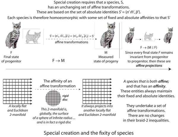
VII.5.12 Figure 45 shows the effects of a population with a proposed deformation retract and that can scale so that S’ = {φn, φm̅, φp̅} = φ{n, m̅, p̅} = {φn, m̅, p̅}. It can in other words change in its numbers, with no effects on any other variable, and so that there is no Darwinian fitness, competition, or evolution. This is the creationist and fixity of species proposal.
VII.5.13 The population in Figure 45 can change n with zero effects on m̅ or p̅, so that if we have n copies of entities, all sharing m̅ and/or p̅, then we expect M = nm̅ and P = np̅ to hold at all possible points, over all generations, and whether we measure them over T or τ.
But this is the proposal that biological populations are always “collinear”. It is the proposal that if we use an index i = 1, 2, 3 and consider the three points (xi, yi, zi) in a Euclidean realm, then the ratios spanning (x1, y1, z1) and (x2, y2, z2)—which are (x2 - x1) : (y2 - y1) : (z2 - z1)—are equal to the ratios spanning (x1, y1, z1) and (x3, y3, z3)—which are (x3 - x1): (y3 - y1) : (z3 - z1). Or alternatively, the triangular (xi, yi, zi) area is zero so that x1(y2 - y3) + x2(y3 - y1) + x3(y1 - y2) = 0. All rates of change are constant.
As suggested in Figure 45, the “indifferent to n” collinearity proposal is that all possible configurations involving n end up invariant. All possible combinations and figures have the same angles, areas, and perimeters when projected along any axis involving n. All figures remain parallel; all angles and ratios remain the same; and all commodities demonstrate the same rates of change.
VII.5.14 All configurations and permutations involving n form a set of affine transformations that can be translated along any plane, and without any change. Since their transformations and projections perform exactly as they did before, then they are all also “coplanar”.
VII.5.15 If biological populations are indifferent to numbers, so that M = nm̅ and P = np̅, then they are always self-similar in n. The number dimension must have D = 1, such that no matter how often we scale and replicate in space and time, the population remains the same. It can accomodate exactly the same types of entities, which will then replicate in the identical fashion. Biological populations and the set A must then have the same self-similarity as a Euclidean line.
VII.5.16 The number of entities, n, in any population, is also a in A. It is injective into both B and C. And since B and C are both surjective over A, then they must both also have the fractal dimension D = 1, and so that when they are each associated with A, they each produce D = 2. They must both therefore be mutually linear with respect to n. Since they each have the self-similarity of a Euclidean line, it is preserved when they associate. This population must be perfectly Euclidean.
And since A, B and C have these collinear, injective, and surjective relations, then when the three associate with each other they exhibit D = 3, and preserve their Euclidean self-similarity.
VII.5.17 But if A, B, and C are linear with respect to each other, so they can all be indifferent to changes in n, then since the gradient in numeracy is ∇Q = (nfinal - ninitial)⁄N, it must be zero. We always have nfinal = ninitial or the equivalent, which is both a zero gradient, and a rate of change of gradient of zero. So we have nfinal - ninitial = 0, ∇Q = 0, and d∇Q = 0.
VII.5.18 The divergence in numeracy, ∇ • Q = m̅final - (m̅initialninitial ⁄nfinal), must also be zero. Since n never changes, then m̅initialninitial = Minitial, while m̅finalninitial = Mfinal meaning that since M is linearly related to both n and m, then if there is no change in n there can be no change in either m or M, so we always have m̅initial= m̅final. So if n does not change, then neither does the population’s mass at any point. Both the divergence and its rate of change are zero.
VII.5.19 And then also granted that the curl in numeracy is ∇ × Q = p̅finalm̅initial(nfinal - ninitial), then again since ninitial = nfinal, both the curl and its rate of change are always zero because both the divergences and gradients in n and m are zero, imposing the same on p̅.
VII.5.20 Since both A and B are injective into C which is surjective over both, then if A does not change, no more so do either B or C, for A contains their rates of change. So if a population is indifferent to n, so that it is replicatively and self-replicatively linear, then the inevitable consequence is that neither m nor p can ever change. Since M = nm̅ and P = np̅, then both m̅ and p̅ must always have the same rate of change as n. And since the only way to form the various integrals is through the interactions with the surroundings that require dm and dp, then no population quantities can ever form. Those curls and divergences of zero, and their rates of change of zero, mean no change anywhere, at any time, in any population.
VII.6.1 Proving the general case over all manifolds is not enough. We must prove it for each individual one for the absolute time intervals across the manifolds of TN, TM, and TP combine to create a joint T. Their circulation distances τt, τm, and τn similarly combine as τt.
VII.6.2 The set of TN, TM, TP, and T, and the set of τt, τm, τn, and τt coalesce. They are a Lorentzian four-manifold.
VII.6.3 Since the Ts and τs must form the Cartesian product T × τ we immediately have a biological version of the Cauchy tensor. We name it after Ernst Haeckel, a German evolutionary biologist who discovered and named thousands of new species, and who reconstructed evolutionary history based on morphology and embryology.
VII.6.4 The Haeckel tensor is a 4 × 4. Since each generation completes, then we must have τt ⊂ A ⊂ B ⊂ C. Our Haeckel tensor therefore has the following structure:
Table 3
The Haeckel tensor
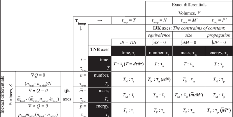
VII.6.5 The tensor rows use the rectilinear ijk axes to project their inexact differentials into the surroundings through their Sn-1 surfaces at each moment t. They do so with the dynamical momentums n, m̅, and p̅, and over the absolute clock times T, TN, TM, and TP.
VII.6.6 The tensor columns use the hyperspherical IJK axes to project their exact differentials through each population’s interior volumes, Vn. They are then a combination of the kinetic plus potential energies projected through the surfaces. They satisfy all of Figure 39’s constant loops, complements, and inverse couplings for the group operations all around the generation of s ◦ s’ = s’ ◦ s = τ and s ◦ s-1 = s-1 ◦ s = S’ that can repeat the same process, with π = [(1 × 1δ=1 → 1)1 ⇔ (1 ÷ 1δ=1 → 1)1].
The columns therefore state the generation distance, and the transformational possibilities, as the sums over sets of minima and maxima as can complete a circulation, and so as the combination of S’ = {n’, m̅’, p̅’}, dS’ = dn’ + dm̅ + dp̅’, and dt = Tdτ—which is T = dt⁄dτ—distributed over the relative generation times τt, τn, τm, and τp.
VII.6.7 The individual tensor components state every value with their TNB Frenet-Serrat unit axes, linking rows and columns, and mediating all ongoing interactions. They form all fibre bundles as Sn-1–Vn-1, Sn-1–Vn, Sn–Vn, Sn–Vn+1, and Sn+1–Vn+1.
VII.6.8 Since we now have all absolute real time values as a set of both inexact and partial differentials, ∂ and δ, with respect to t upon the rows; and all relative and generational values as the exact and also partial differentials, ∂ and d, with respect to τ upon the columns; then the Haeckel tensor’s “principal diagonal” is the set of four combined values plus rates of change as create the T:τt, TN:τn, TM:τm and TP:τp that are the normal stresses. They are the divergences that populations must maintain, over specified intervals, and so to establish the properties and quantities that keep them viable. They span both τ and T using their set of rates and form the deformation retract of S’ = {n’, m̅’, p̅’}. The principal diagonals coordinate the three sets of axes and events.
VII.6.9 Replication is about the different time scales, τ and T, across which the rates of the divergences and curls are projected. The V4 is simply a statement of volume. It is the gongyl distributed across the four dimensions. The four glomes are the rotachoron’s S3 surfaces which state its values. But since these are biological entities, then those time scales have a group operation. Their paths must stay connected. We must maintain both s ◦ s’ = s’ ◦ s = τ and s ◦ s-1 = s-1 ◦ s = S’.
VII.6.10 The proposed affine transformations in Figure 45 and their collinearity can do no more than describe the overall distribution throughout the entire S3–V4 space that is the τtnmp rotachoron. It is an alternative presentation of Figures 33 and 35. It states the normal stresses and principal diagonal for the overall T:τt, TN:τn, TM:τm and TP:τp distribution.
VII.6.11 The principal diagonal is the “isotropic component”, I. It states the overall distribution present in every viable population. It is the mean values and set of divergences each population must maintain as the set of properties and quantities that guarantee its connected and isomorphic paths. It is the set of exact and inexact values that span both τ and T using a set of rates based upon the deformation retract and which also establishes the identity, through s ◦ s-1 = s-1 ◦ s = S’ = {n’, m̅’, p̅’}.
This isotropic component, I, establishes the constant radius, r, that is both dr = 0 and ∫dr = 0 for the maximum possible gongyl volume. It is the set of all possible Hausdorff points within the interior so that a biological space of dimension D = 4 exists at every point whose paths are all connected. They can then form constant loops of s ◦ s’ = s’ ◦ s = τ everywhere, and so that we have both (1 × 1δ=1 → 1)1 and (1 ÷ 1δ=1 → 1)1 for the π equilibrium at all points. We then have both the exact ∫dS = ∫dP = ∫dM = 0 and the inexact ∇Q = ∇ • Q = ∇ × Q = 0 holding good at all points.
VII.6.12 Since every possible population has mean values over every T, then every population has an isotropic component. Every viable population then sees a universe in which its every existing entity can maintain itself over every interval, with that set of mean values.
VII.6.13 A population’s isotropic component forms an S3–V4 rotachoron whose surface is the set of derivatives that are its four τtmp, τtnm, τtnp, and τnmp glomes. These produce the Euclidean realms whose fractal dimensions are each D = 3, and that can therefore extend evenly in all directions. These realms then have their six τtn, τtm, τtp, τnm, τnp, and τmp coplanar and Euclidean slices and surfaces throughout themselves, each of fractal dimension D = 2. And since all are coplanar, then their derivatives are the collinear τt, τn, τm and τp, all of them maintaining their fractal dimension of D = 1. And if they are all collinear over all possible points, then they are each composed everywhere of the Euclidean points S’ = {n’, m̅’, p̅’} whose fractal dimension is D = 0, so they can carry the same invariant entities about their Whitney umbrella s ◦ s-1 loops. It must have ijk = IJK = TNB.
VII.6.14 Every viable population can use a set of divergences and curls to create such a realm and realmspace over time, which is then a V4 gongyl with its S3 surfaces, all with ijk = IJK = TNB.
VII.6.15 Although every viable population must have an isotropic component, that same isotropic component is the set of mean values that are its divergences over its every interval. However … if n is indeed proposed as invariant, then the fixity of species immediately suggests that those are the actual values for the actual entities maintained throughout all populations, and at all times.
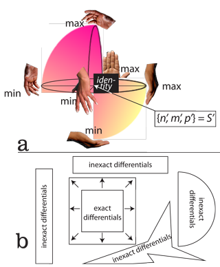
VII.6.16 The sum of every tensor’s off-diagonal and shear stresses is its “deviatoric component”. They are the deviations from the means. They create a population’s “deviatoric stresses”.
VII.6.17 A population’s deviatoric stresses are its curls. They are its changes in its gradients, and its divergences, ∇ and d∇, about any circulation. So if we gradually move towards the mean, at any point, then the deviatoric component equally gradually disappears … only to reappear if we either continue on past the mean on the other side, or turn and move back to our start point. Each is away from the mean.
VII.6.18 Although the deviatoric component always has ijk ≠ IJK ≠ TNB, its stresses invert. They help ensure that everywhere maintains s ◦ s-1 = s-1 ◦ s = S’ = {n’, m̅’, p̅’}.
VII.6.19 Since the deviatoric stresses invert to sum to the isotropic component, I, then they form a Möbius strip; a real projective plane; and an identification space.
VII.6.20 The TN:τn normal stress for numbers in Table 4, underneath, is a part of the isotropic component. It is the principal determiner of the ∇Q = (nfinal - ninitial)⁄N gradient in number.
VII.6.21 The TN:τn normal stress also helps establish the divergence and the curl in numeracy. It therefore holds the mean values in number for each of ijk, IJK, and TNB. One set comes from each row in its 21 constitutive elements.
VII.6.22 The gradient in numeracy is also determined by the deviatoric stresses on both its row and its column. The τm and τp on its row state the current circulation rates in m and p. The sets B and C exhibiting them are surjective over the A that holds the entities. They therefore affect all replication and self-replication times.
VII.6.23 But the dual TN:τn index also means that TN is the principal determiner for the constraint of constant equivalence that forms its column. This has ∫dS = 0. It sets the overall rate and is a Boy’s surface meridian.
VII.6.24 The constraint of constant equivalence has two other determiners. They are the TM and TP that also associate, in that same column, with τn. Since they are off-diagonal, they are deviatoric stresses. Since B and C are again surjective over A, then the τn that establishes the overall circulation amounts in n are affected by the absolute times that T, TM, and TP each establish. Those will help determine the ultimate replication and self-replication behaviours found in A.
VII.6.25 The combination of rates and times that forms the normal stress and isotropic component of TN:τn that determines the overall population numbers and changes in numbers is composed of the following 21 elements:
Table 4
The 21 elements in the TN:τn (n⁄N) isotropic component
|
3rd derivative |
2nd derivative |
1st derivative |
mean |
1st |
2nd |
3rd |
||
absolute time, |
← ijk |
d3n⁄dt3 |
d2n⁄dt2 |
dn⁄dt |
n |
∫n dt |
∬n dt dt |
∭n dt dt dt |
min–max |
↑ IJK |
d3n’⁄dN3 |
d2n’⁄dN2 |
dn’⁄dN |
n’ (=n⁄N) |
∫ n’ dN |
∬n’ dN dN |
∭n’ dN dN dN |
relative time, |
■ TNB |
d3sn⁄dτn3 |
d2sn⁄dτn2 |
dsn⁄dτn |
sn (=n⁄τn) |
∫ sn dτn |
∬sn dτn dτn’ |
∭sn dτn dτn dτn |
VII.6.26 As is the TN:τn isotropic one, every tensor component is a confluence of various quantities as (a) integrals, and (b) derivatives or rates of change. The derivatives and rates build the quantities in the integrals. The different integrals are formed from different sums over different limits. These are: (i) from 0 to T, which are the intervals of time for the horizontal row and that use the ijk axes; (ii) between a minimum and a maximum and so across the population’s entire range for the vertical column in their tensor and that use the IJK axes; (iii) 0 and 1, to link volumes and surfaces, and the beginnings and ends of the circulation as a discrete set of events using the TNB axes.
VII.6.27 Every tensor component therefore states both an amount and a rate. This is always both (a) the amounts, and (b) the times over which they are acquired and/or consumed. This is also always in all of their 0, 1, 2 and 3 dimensions, involving all manifolds and dimensions, and the ijk, IJK, and TNB axes and their means and distributions.
VII.6.28 Given the above, then every tensor component is a contributor to a Lorentzian four-manifold. Each is multiply-connected timelike to all others through both its row and its column. Any change in any one manifold has a timelike influence on all others. It changes the absolute time periods, T, they each take to traverse their τn, τm, and/or τp distances, as well as the amounts concerned. Populations can thereby impose different magnitudes and rates on each other through their zero-, one-, two- and three-dimensional retracts and hyperplanes. All these can occur in response to -∂n⁄∂t … and such as we measured in our Brassica rapa experiment.
VII.6.29 Every diagonal component in the Haeckel tensor is an isotropic component. It is a normal pressure. It also has four parts. It is:
• a set of quantities, which are integrals;
• a set of rates, which are their derivatives, as divergences and curls.
These are each stated both:
• absolutely;
• relatively.
VII.6.30 Each component in the tensor also has its TNB axes responsible for creating its timelike connections by (a) projecting its numerators horizontally along its rows for its rectilinear ijk values; and also (b) by projecting its denominators vertically up its columns for its IJK hyperspherical ones.
VII.6.31 Each component projects a scalar. Each helps create its overall rank zero tensor. Each thus has a definite and distinct magnitude. In the case of the TN:τn component, this is n as the number of entities in that population, at that time.
VII.6.32 Each tensor component also helps create a mean. This is a part of a range between a minimum and maximum. In the TN:τn component, it is N as the mean across that interval.
VII.6.33 And finally, each tensor component helps create a generational expanse. This is the set of values that carry it all about a generation. It is the distribution between 0 and 1 that crosses a real projective plane, thus also moving towards infinity and so some maximum. In the case of the TN:τn component, there is a specified number of entities, n, at every t.
VII.6.34 And since the product A × B × C must exist, then each of those n is an a in A, injective into a discrete collection of n bs in B, and into n cs in C. It is therefore a mixture of all three ijk, IJK, and TNB axes; and all three types of fractal measures, with D between 1 and 2, 2 and 3, and 3 and 4 for each manifold and combination thereof.
VII.6.35 The axes associate pairwise over all combinations. Since xy is not the same as yx, each component contributes to a tensor of rank one. Each thereby gives a sense of direction towards, and away from, its mean, which is the isotropic component, I. This is a vector.
VII.6.36 Each component always transforms to give a sense of being closer to or further away from some given mean value, and closer to or further away from the beginnings and ends of a generation, τ.
VII.6.37 Every tensor and tensor component also always has a gradient, ∇, towards and away from whatever mean; and towards and away from the beginnings and ends of that generation. Both these gradients can change in their amounts and rates, and so as ∇ , d∇, d2∇, and d3∇.
VII.6.38 Every distinct value in every tensor component is always (a) an event at some instant, t; (b) some proportion of some mean; and (c) located at some point between 0 and 1, and so over τ. Each is therefore always either less than or greater than its mean; moving towards or away from that mean; and over intervals with specified rates. Those are (a) absolute, (b) with respect to that mean, and (c) at a given location in the generation.
VII.6.39 And since we have both xy and yx, then these gradients and their changes form a group, complete with the inverses and the identity that create an identification space. The various axes drive their means and their attributes through the generation.
VII.6.40 There are first, second, and third integrals over each set of axes. Their lower and upper limits move them over T and τ, also creating the population magnitudes N, M, and P. They accumulate using their gradients and changes in gradients, their divergences and changes in divergences, and their curls and changes in curls. Their matching derivatives state their rates. These together establish the compete set of behaviours for each generation. They are also invertible.
VII.6.41 The TN:τn component creates both N and τ. This is numbers maintained both (a) at each point, t, and (b) in succession about the whole circulation. There are again always both (a) magnitudes; and (b) rates.
VII.6.42 By the Church-Turing thesis, the final result of any tail-recursive function appears identical to a loop, and conversely.
VII.6.43 Every isotropic component upon the diagonal uses its rectilinear, absolute, and temporal ijk axes to establish the momentum value for its row. They are directly observed. These are the biosurfaces S0,1,2,3. The sum of all the row offerings, for that ijk value, is a set of loops.
VII.6.44 Every isotropic and diagonal component also uses its hyperspherical and relative-proportional IJK axes to establish enegy and circulation value for its column. This magnitude ranges between a minimum and a maximum. It is the biovolume, V1,2,3,4. The sum of all the column offerings, for that IJK value, is a recursive function.
VII.6.45 Every deviatoric and off-diagonal or shear component interacts with two principal diagonals:
• It interacts horizontally to influence the isotropic component that carries the means for its row. It therefore affects that set of absolute clock times, T.
• It interacts vertically to influence a second isotropic component in its coumn, and so to influence a set of relative and successive generational circulation lengths, τ.
VII.6.46 The deviatoric component interactions are the curls and the partial differentials that create all changes in both τ and T. Their values sum to zero for the exact differential and principal diagonal.
VII.6.47 Each deviatoric component affects the isotropic one on its row with its numerator.
VII.6.48 Each deviatoric component affects the isotropic one in its column with its denominator.
VII.6.49 Since a biological circulation is a Lorentzian manifold, then a population’s responses to the -∂n⁄∂t events that are losses in numbers as jerks will contain opposite effects from each deviatropic component affecting it. Each one affects it in opposite and matching ways, but absolutely and instantaneously in one aspect, and relatively and successively in the other.
VII.6.50 Any change in numbers affects both a row and a column. It is therefore a net loss in structure. The loss in a row as TN is an absolute loss at some moment, t. It has a sense of direction. It moves either from above the mean towards the mean, or else from the mean and closer towards zero. It is therefore a vector expressed absolutely in time.
VII.6.51 The loss in a column as τn is a loss expressed as the flattening of a temporal gradient. It is therefore also a vector, with a sense of direction, and all across a circulation.
VII.6.52 The jerk of j = -∂n⁄∂t, as the loss in numbers, is a group operation involving the deviatoric component. It carries the τn gradient closer to the mean. It therefore drags the rate of activity in mass and energy, as TM and TP, closer to its mean.
VII.6.53 We have already met the deviatoric components TM:τn and TP:τn. They are the changes in rates and gradients that are Maxim 3 of succession, and Maxim 4 of apportionment. They produce ∇ × M = ∂m̅⁄∂t - ∂n⁄∂t and ∇ × P = ∂p̅⁄∂t + ∂W⁄∂t - ∂n⁄∂t respectively.
VII.6.54 The curls result from the partial differentials exhibited in n = M⁄m̅ = P⁄p̅. Since n has both m̅ and p̅ as its denominators, then any ongoing changes in numbers will produce opposing changes in them both; as also will any ongoing changes in them be opposed to changes in numbers.
VII.6.55 If the jerk as the ongoing losses in numbers is negative, then the curls as changes in m and p will be in opposition to n, and so will be positive for the circulation … and as in the braid-3 dS’ = dn’ + dm̅’ + dp̅’ of Figure 19c.
VII.6.56 And contrariwise … whenever population numbers increase, there is a decrease in the average individual mass, m̅, and the average individual energy, p̅, and for exactly the same reasons.
VII.6.57 However … the deviatoric τn responses to any -∂n⁄∂t also affect the head of their column. This is the T that establishes the overall generation length.
VII.6.58 Since this is a multiply-connected timelike Lorentzian four-manifold; and since the temporal gradient has flattened; then the rate at which time flows through this population slows. The generation length, T, extends through τn.
As in Figure 40, all losses in numbers will therefore push the population to the right of the small τnmp and τtnp glomes at top left and centre. This decreases numbers and energy density, respectively. But the population is also pushed to the right of the small τtnm and large τtmp one, which increases masses and generation times, again respectively. We measured exactly these effects in our Brassica rapa experiment.
VII.6.59 Since a generation is a four-dimensional τtnmp rotachoron, then if biological populations are truly indifferent to numbers, they must never move in the n-direction. This is therefore the demand that the rotachoron transforms to a spherinder by flattening on an n-hyperplane. The population is now obliged to follow Figure 40’s cubindrical path with the large black arrow. This is the path directly towards the τnmp numeracy glome. The rates are fixed at the τtmp equator. They are set to n = M⁄m̅ = P⁄p̅ through τn.
VII.6.60 Since n is now invariant, then τn is also invariant. The population has ninitial = nfinal = nmean at all times. Population changes in M and P must therefore track the average individual values, m̅and p̅.
VII.6.61 The indifference to numbers is the formal request that the curl in numeracy of ∇ × Q = p̅finalm̅initial(nfinal - ninitial), be zero. But this again means that m̅ and p̅ must abide by Figure 45. They must have fractal dimensions D = 1 and be collinear and coplanar. They must both follow their divergences exclusively. They may not have curls, for all those are caused by τn working through ∂n⁄∂t. But since n does not change, then only the isotropic components are possible. There can be no shears.
VII.6.62 These demands are all measurable. Therefore:
• if m̅ and M change at different rates; or if
• p̅ and P change at different rates; or if
• generation length, T, changes …
then the population is not exclusively isotropic. It is not free from changes in numbers. A deviatoric component exists.
VII.6.63 Figure 45 has also already demonstrated that if a population is indifferent to changes in n and so has a flat and Euclidean fractal dimension and self-similarity of D = 1 in one dimension, then it will have the same D = 1 in the others. This invariant self-similarity therefore affects the t-manifold. The indifferent to numbers demand is therefore the demand that the t-manifold cease creating a multiply-connected and timelike space. The tn, tnm, and tnp time flows must therefore retract to a single identity. All timelike connections will become simply-connected. They will all relocate to the generation midpoint, τ’–t’.
VII.6.64 The request that a population be indifferent to numbers is therefore the request that a rotachoron convert to a spherinder, and that the entire V4 volume collapse onto an S3 surface.
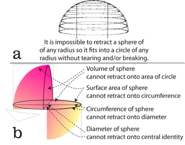
VII.6.65 If a population is indifferent to numbers, then it has no rates in n. Since τt vanishes then the τtnm, τtnp and τnmp glomes must collapse in the n-direction. This therefore becomes the demand shown in Figures 46a and 46b. The glome surfaces of τtn, τnm, and τnp must keep collapsing. The rotahedrons flatten to rotagons. But since—as the values for their fractal dimensions makes clear—each Vn volume is larger than its equivalent Sn-1 surface, then this is impossible. It cannot be done without breaking or fracturing.
VII.6.66 The actual flattening may in principle be impossible, but the fixing of values and rates is not. So the demand that populations be indifferent to numbers is the demand that all rates tend to an equality. All divergences and curls must be zero. All possible populations must strive to set their S0 inputs identical to their outputs. They become scalar multiples of each other. All their molecules and energies are left in an unchanged and unchanging condition. Generation times also become fixed and unchanging. All populations tend to the S’ = {n’, m̅’, p̅’} values that define the τ’–t’ generation midpoint. Thus the proposed n-retraction creates an infinitesimally small and closed timelike loop located at the generation midpoint … which is a “singularity”.
So we again find, thanks to our topological investigation, that the proposal that biological populations are indifferent to numbers makes all biology impossible, for it is the demand that they all form fixed and rigid discs incapable of homeomorphisms and transformations. Figure 45’s proposed affine transformations of S = φ{n’, m̅’, p̅’} and S = {φn, m̅, p̅} are therefore again impossible.
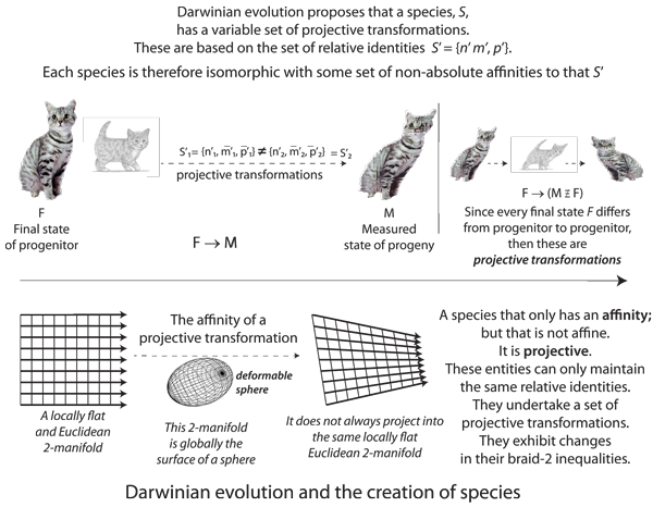
VII.6.67 The only remaining possibility, for all biological populations, is the projective transformations of S = a{φn, κm̅, χp̅} shown in Figure 47. They must form the deformable spheres in Figure 48a, and that can deform, in all directions, over time. Figure 45’s affine transformations of S = {φn, φm̅, φp̅}, S = φ{n, m̅, p̅} and S = {φn, m̅, p̅} are impossible because they demand an equality in rates in n’, m̅’, and p̅’ … which is a rigid disc. Biological populations must, instead, exhibit the different curls and divergences for the sphere in Figure 41b. As in Figure 48a, they must form the spheroids that can freely stretch and flex, in different ways, under scaling. So if any population is to scale by some α, then the φ, κ, and χ that establish the scalings in each of n, m, and p must differ.
VII.6.68 We have already proven that every population has a universal covering space, C, and a base, B, whose fundamental groups, π(B), are homeomorphic with the cover’s deck transformations, η, and so that the cover’s surjective ξ projections are the inverse of the base’s injective fibre lifts as ξ-1; and also such that η ◦ φ = φ ◦ η = φ. This then means that η ◦ κ = κ ◦ η = κ and η ◦ χ = χ ◦ η = χ, so that none of a population’s transformations affect the deck transformations. And since the universal covering space is also a mapping cylinder, then all those homeomorphic and isomorphic cylinder mappings Mλ:A ↔ B, Mλ:A ↔ C, Mλ:B ↔ C, and Mλ:X ↔ Y involving the progenitor domains, X, as preimage, and progeny codomains, Y, as image, exist. So also do all open Hausdorff sets and connected paths. They exhibit the appropriate absolute and relative times and circulation distances, which are the interactions with the surroundings. Their inbuilt Chomsky production rule, δ, governs them all.
VII.6.69 No matter how circuitous the perimeters in Figure 48b, we can summarize them all as one-dimensional line expanses. They will all end up ‘x metres long’, and no matter how varied their shapes and paths. The areas will all similarly end up as ‘x square metres’, and again no matter what their shapes.
VII.6.70 We can scale the square in Figure 48b by any arbitrary factor, ξ. It will hold its properties and proportions. That scaling is now a projection. It is a self-replication and a set of exact differentials.
VII.6.71 If we scale the square by ξ, we can then deform it with a set of inexact differentials. But as long as their sums form a group, then (a) the area to perimeter proportions will remain constant; (b) we can recover the original square at any time. We simply reverse the transformations. This is the inverse fibre lift, ξ-1. We have ξ ◦ ξ-1 = #. The inexact differentials have formed a suitable group.
VII.6.72 The above square transformations are between two dimensions, and hold as a matter of principle for any two. For example, virtually the only thing that grows in the harsh northern environments of the Arctic circle and steppes is lichen. Almost the only thing that will eat the lichen is the reindeer. But they must urinate ten to twelve times daily. This is a considerable loss of valuable salt. They therefore drink their own urine. Siberian sled masters often urinate by their sleds to attract reindeer there to hook them up. A traditional Inuit hunting method is to cover a large hole with thin slabs of ice; to urinate on a trail leading to the trap; and to wait for the reindeer, seeking salt to lick, to walk right up and fall in.
The poronkusema is a traditional Finnish unit of measure that is the approximate distance a reindeer will walk between its urination events. The poronkusema is approximately six miles, 9.6 kilometres, delivering approximately 1.2 litres of urine. We can round this and bring two dimensions together so that 1 poronkusema = 10 kilometre-litres.
We now consider a Reindeer 1 that walks 20 kilometres to produce a ½-litre of urine. This is equivalent to a Reindeer that 2 that walks 5 kilometres to produce 2 litres. And both are equivalent to the more standard Reindeer 3 that walks 10 kilometres to produce 1 litre. Each is a poronkusema derivative with respect to distance. The urination rates and distances walked, looked at in isolation, seem to vary. However, they all sum, over their respective distances, to produce the same integral.
VII.6.73 The heart of biology and ecology is Figure 8’s Hooke cell which is a Whitney umbrella and our S’ = {n’, m̅’, p̅’} deformation retract. It can undertake a simultaneous fibration and cofibration, involving both x and y, and so that for every x there is a +y and -y, while for every y there is a +x and a -x for an identification space.
VII.6.74 The Hooke cell is an identity operation. It is always x + 0 = 0. It leaves the original unchanged. It also abides by the first law of thermodynamics.
VII.6.75 When we take measurements, we extract, and then replicate, every atom and joule in any arbitrary entity. We generate and regenerate the original. This is an identity operation. We simply take our Hooke cell as a standard to create our plessist.
VII.6.76 We can now create that Hooke cell. We first note that the Earth receives a solar energy, at temperature latitudes, that is of the order of p = 100 joules per second. We can take this as a reference energy rate for our reference Hooke cell. We therefore set it as p* = 1. So if some arbitrary biological entity absorbs and emits energy at n times that rate, then it is equivalent to n Hooke cells. We measure it as np*. We have created our plessist. It replicates all the original’s behaviours.
VII.6.77 We have successfully used our Hooke cell in an identity operation. We can at any time reverse this process. We have left the original completely unchanged.
VII.6.78 We next observe that the average terrestrial eukaryotic cell has a mass of m = 10-12 grams. We take this as the reference for our Hooke cell. We set it as m* = 1.
By the first law of thermodynamics, which our Hooke cell enshrines, we can now measure any arbitrary entity; determine its mass; undertake our identity operation; and declare it as nm*.
This is another identity operation. It has left the original unchanged. But … it has accorded a specified mass to our plessist, which can take any value without changing its behaviour.
VII.6.79 Our plessist may have the above np* energy intake rate, but it must also always have some energy content or enthalpy. At a representative 25° Celsius, the average biological organism contains matter whose thermal energy is of the order of 0.5 kcal per mole. Glycine, for example, has an energy content of approximately 979 kilojoules per mole (Haynie 2001). We can therefore declare that our Hooke cell always contains 1,000 kilojoules per each mole of its constituents. So in yet another identity operation, we can measure any arbitrary entity, and then transfer it as a specified energy density of nV*, and so as some multiple of our reference, to our plessist. This is another identity operation.
VII.6.80 We can then declare that our Hooke cell takes T = 1,000 seconds to go through its cycle of surrendering and replacing every molecule and joule. This is now our reference generation length. We set it as T* = 1. Our Hooke cell replicates itself after that interval. We can again replicate any other entity’s generation length, in yet another identity operation, leaving that original unchanged. Granted that a blue whale, for example, has the generation length T = 31 years, then compared to the Hooke cell its length is T* = 11,315. This simply means that where the blue whale replicates itself once only, our Hooke cell does so 11,315 times, using exactly the same quantity of energy.
VII.6.81 And finally, we create a biological population by taking up 1,000 of our Hooke cells. If we keep the number constant over any period, T*, then we have a population of plessemorphs that can substitute for whatever number of plessists recognizes that as an average. Whether as an a1 or an aa in A, they can interact with the surroundings using a specified quanty of mass, numbers, moles, and energy, over 1,000 seconds, creating our π = [(x × 1δ → y)T1=1 ⇔ (y ÷ 1δ → x)T1=1] unipollent equilibrium.
VII.6.82 Our 1,000 plessemorphs have linked a known and determinable biological population directly to a set of molecular components, in terms of a standard mass, energy and molecular composition … all undergoing reproduction at a known rate. Since the Greek for species is genos, then mass, energy, numbers, and generation length join together to describe an entire population in an “engenetic constant”, Ω.
VII.6.83 Our engenetic constant, Ω, is simply our unit rotachoron. It stretches exactly one unit in all its four directions, maintaining a πequilibrium, ijk = IJK = TNB, and an equality between exact and inexact differentials everywhere throughout itself.
VII.6.84 Since we can describe all populations relative to our engenetic constant, we can compare them to each other. We simply scale our unit rotachoron with its exact differentials, and its deformations produce a matching set of inexact ones. We are therefore free to introduce and to remove entities, and to adjust their masses and energies as a set of plessists. They can vary, however we so choose, around the plessemorph mean that is our unit rotachoron and engenetic constant. These comparisons are integrals and derivatives in the various dimensions: both exact and inexact. At the end of any such operation, we can then compare our proposed plessists to the real world entities we began with, and note any differences in values.
VII.6.85 We already know, for all those transformations, that both dt = Tdτ, and dS = dn + dm̅ + dp̅ must describe our equilibrium population. Our reference one of plessists and plessemorphs, with their a in A, b in B, and c in C, must also satisfy:
dS = χ(dm̅*⁄m̅*) + ΩT*(dV*/V*),
and/or:
dS = κ(dm̅*⁄m̅*) + ΩT*(dP*/P*).
where we always measure across the population as V * = M*/P*. The values for κ and χ are always stated in joules. However we choose to deform our population and rotachoron, they can scale m and p, respectively, as κm̅ and χ p̅.
VII.6.86 Our plessists and plessemorphs are completely predictable. We can compare them to any population at any time.
VII.6.87 By the first law of thermodynamics, if a given generation is to complete, then although κ and χ are free to vary, there must be equilibrating changes all around that given circulation. The values κ/χ and 1 - (χ/κ) must maintain a constant relationship. If one changes one way, the other must change another.
Again by the first law of thermodynamics, the energy any one population of plessists uses to change its mass, m*, and/or numbers, n, and/or energy density, V*, and/or generation length, T*, is precisely equivalent to some corresponding change in some other. We can transform to and from any population while always leaving the original unchanged.
VII.6.88 If a population is indifferent to changes in its numbers so that dn = 0, then they must produce the sphendrical and cubindrical values with those rates of change. Those are the dχ = dκ = 0 transformations in which κ and χ remain invariant. They therefore produce those ΩT’(dV/V) and ΩT’(dP/P) population values that always change at the same rates as the individual m̅* ones.
VII.6.89 All the above claims about fixity of species can now be easily tested by experiment. Brassica rapa failed, utterly.
VII.6.90 The same theoretical and experimental results tell us that if populations do indeed exhibit Darwinian fitness and competition, then we will have a deformable rotachoron. Our values for κ and χ will vary with φ and α, meaning that the ΩT’(dV/V) and ΩT’(dP/P) terms will also vary—but in their associated ways—over the generation. And since they varied in precisely those ways for Brassica rapa, then all its transformations have a curl. All its deviatoric stresses sum to an isotropic one. It is proven sensitive to changes in numbers.
And not only did Brassica rapa’s generation length vary between 28 and 40 days, but we measured the transformations caused explicitly by dκ and dχ at 3.28 grams of mass and 54.012 joules of energy, per 1,000 plants. Those values are the deviatoric components as the offsetting to the changes in the masses and energies of seeds produced per each pod, and plants produced per each pot, as population numbers changed.
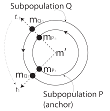
VII.6.91 Only the Möbius strip remains. If a given species is proposed as isotropic and independent of all influence in numbers; and if it contains the two Supopulations P and Q; then they each face the immediate difficutlies of their fractal dimensions being D = 1. Since they must be affine, they must each transform as the rigid disc in Figure 49. Their divergences must maintain a set relationship. Their curls must be zero. If their initial values, at t-1, have a given relation to the generation mean, then all their values must have that relationship at all times. They must be as shown at all subsequent points, t1. One population is an “anchor” by being consistently closer to the mean. It must preserve the S’PQ identity not ony by having the smaller magnitudes, but by having the smaller ranges and rates.
If Subpopulation Q has three times the mass at one point, it must have one-third at another. Whatever value Subpopulation P has closer to the mean, both it and Q must maintain those specific rates of change, so their inverses fall within the identification space.
Since Subpopulation P and Q are members of the same species, then their generation lengths must be directly proportional to their masses and energies … and must remain static. Any variations either across or between generations is a curl and a deviatoric component.
All this can also be subjected to testing by experiment. Brassica rapa exhibited a measurable deviatoric component. It did not hold to those proposed values. It was not a rigid disc, but a deformable one.
VII.6.92 We can now benefit from the advantages of our topological approach. If a homeomorphic mapping from A to B exists; and if B can access neighbourhoods in its mapping cylinder, Mλ; then A can use its identity, S’, to map to those same neighbourhoods in that same mapping cylinder; with the same holding for B if a homeomorphism exists from B back to A; with the two then accessing each others’ mapping cylinders, which are the surroundings. And since they are both simply connected, then those same surroundings are a universal covering space. All events in them are deck transformations, η. They are also the Chomsky production rule, δ. They govern all possible transformations within the population, which act as a base with homeomorphic fundamental groups.
VII.6.93 Euler established topology by solving the Knigsberg Bridge problem. He demonstrated that the fixity of shapes proposed in Figure 49 is irrelevant in solving certain very general problems. He elucidated the four important principles that:
• the size and shape of each landmass is irrelevant;
• each landmass can be reduced to a single vertex.
• the number of vertices is critical;
• the length of the bridge connecting each vertex is irrelevant.
VII.6.94 Topology is centred on the deformation retract. As in Figure 50, if biological populations are to successfully replicate, then they must abide by all four of Euler’s principles. They must have:
• maxima and minima in n, m, and p whose ± values act as topological vertices;
• variable generation lengths, T, that act as multiply timelike connecting and topological bridges between the above;
• variable flux amounts in N, M, and P—the latter two satisfying M = nm̅ and P = np̅—built from the variable ranges in in n, m, and p, and also from the variable times and rates in t and T, for variable circulation lengths, τ.
• a set of magnitudes, each of which can be reduced to a single value, for a set of vertices, and as the deformation retract, S’ = {n’, m̅’, p̅’}, all values maintained at τ’.
VII.6.95 We can also express a circulation of the generations by saying that it is a Chomsky grammar such that the intersection of every n-ball with its retract n-1 hyperplane produces an n-1–ball, with any lower-dimensioned Sn-1 object flattening some immediately higher Vn dimension, that Vn object in its turn being a Vn-1 ball surrounded by an Sn-2 surface.
VII.6.96 A population and a generation are also a Whitney umbrella. They thus provide an identification space that is an irreducible and real analytic set, never singly pure-dimensioned, complete with its pinch points and antipodal -r and +r, and recurvatures. It has the radial and the circulating field principles that are both homomorphic and homeomorphic, creating all syntaxes, semantics, and cyclic groups with their neighbourhoods and identities.
VII.6.97 A biological generation is further the helicoid presented in Figure 9. Our Brassica rapa experiment found that the smaller plants and seeds, as a Subpopulation P, always developed at the most rapid rates. They would initially occupy positions upon the helicoid inside. They would then gradually drift to the outside as those rapid rates increased their various magnitudes.
Our experiment also found that the larger plants and seeds, as a Subpopulation Q, always developed at much slower rates. They would initially occupy positions upon the helicoid outside. But they would then gradually drift over to the inside, as their decreased rates of propagation held them relatively static. This is the inversion of values that creates our Möbius strip.
VII.6.98 If a population is to maintain its essential characteristics, in the face of these opposing sets of magnitudes and rates, then neither of dSP’ = dnP’ + dm̅P’ + dp̅P’ nor dSQ’ = dnQ’ + dm̅Q’ + dp̅Q’ may diverge too widely from each other.
VII.6.99 The above also requires that our ijk, IJK, and TNB axes differ. This requires a deviatoric component, and so a set of Darwinian variations.
VII.6.100 If we set s = nS’, then each distinct entity in each subpopulation is an sP and an sQ, and where that s now also states the current number density found about each. Each distinct s in S must now hold sufficiently closely to their joint sPQ mean, which now means the same numbers of neighbours. Both their rates and quantities must match their number densities. And if we measure over the entire population—and so for the time period T, and the circulation length τ—then this sPQ with its mean number and number density is our plessemorph.
Each distinct plessemorph is now a path, s, in the biological space, S. Each one abides by the two group operations s ◦ s-1 = s-1 ◦ s = S’, and s ◦ s’ = s’ ◦ s = τ. So if some s in sP is to one side of some s in sQ at one point, then each must be the other side of the other at their identification space’s opposite point; and the numbers surrounding each must also invert to create the population mean. The rates in both magnitudes and numbers in dtP = TPdτP and dtQ = TQdτQ form the overall dtPQ = TPQdτPQ. Their inversions form an outer and an inner boundary which together define the mean values that are the axis and the central band upon the helicoid.
The interactions between sP and sQ are the set of braid-3 flips we met in Figure 19. If one variable in dS’ = dn’ + dm̅’ + dp̅’ increases the other two must decrease. That central and most characteristic band that forms the helicoid axis and centre is the deformation retract. We measured its net biological processing, for Brassica rapa, at T =36 days. This again requires that the ijk, IJK, and TNB axes change in different ways to construct a deviatoric component.
VII.6.101 We can express this by saying that if a homeomorphism exists that allows A to access neighbourhoods in its mapping cylinder, then B can use its identity to map its elements to those same neighbourhoods in that same mapping cylinder. And if a homeomorphism exists that in its turn allows B to access neighbourhoods in its mapping cylinder, then A can use its own identity to map to those same neighbourhoods in that same mapping cylinder. Since these two populations can access each others’ mapping cylinders, then an identification exists such that the progenitor domain A(X) can deform the progeny codomain B(Y); while the progenitor domain B(X) can reciprocally deform the progeny codoman A(Y); with each successively using the values n, m, p, and t in each. This is again a declaration of Darwinian fitness and competition.
VII.6.102 For as long as the entities follow the four laws of biology of (1) existence, (2) equivalence, (3) diversity, and (4) reproduction; and the four maxims of ecology of (1) dissipation, (2) number, (3) succession, and (4) apportionment; and the three constraints of (1) constant propagation, (2) constant size, and (3) constant equivalence; then they will all be homomorphic and so homotopically equivalent. They will possess rates that are divergences and curls. But they can only be homeomorphic and isomorphic, and so members of some given species, if they hold to the same deformation retract values, constructing a shared set of exact differentials. They will then also share the same inexact differentials; be constant topological neighbours; and use the same κ to govern their masses and changes in mass, γ, and the same χ to govern their energies and changes in energy, ψ.
VII.6.103 The Church-Turing thesis may well assert that loops and recursive functions can achieve the same effects, but they are not identical. And since they are not identical then they are not perfectly interchangeable between bases and universal covering spaces; or between mapping cylinders and deformation retracts; or between exact and inexact differentials.
VII.6.104 Only those biological entities that are constant topological neighbours can share both average magnitudes and average rates of change, and so be constantly homeomorphic and isomorphic. These constant neighbours—which are plessists—also respond to all changes in numbers. This is again Darwinian fitness and competition.
VII.6.105 A species is a population that maintains a given set of exact differentials and their deformation retract equivalent to a given set of inexact differentials and their curls.
VII.6.106 We know from Newton that maintaining a constant n all around a circulation, to maintain such an equivalence in exact and inexact differentials, requires an acceleration, which is then d2n⁄dt2. A change in that acceleration, as a sudden loss in numbers, is a jerk as j = d3n⁄dt3. But as we have already proven above, the population simply deforms inversely to any such jerk, instituting changes in m, in p, and in T to preserve that equivalence … and as we measured for Brassica rapa.
VII.6.107 Although all jerks are absolute as j = d3n⁄dt3 they can also be expressed relatively, and so as both (a) changes in numeracy, Q, and (b) relative to some specified generation length, and so as dQ⁄dτ and d2Q⁄dτ2. And since these immediately involve permutation in φ, κ, and χ, then they are statements of Darwinian fitness and competition.
VII.6.108 Although the final result of any series of tail recursive functions, as an expression of inexact differentials, always appears identical to a loop as an expression of exact differentials, they are again not perfectly interchangeable. Loops require that numbers do not change. But our Brassica rapa experiment demonstrated that the individual values m̅ and p̅ change at very different rates from the population values M and P, meaning they each have rates of change that are entirely dependent on the rates of changes in numbers. Mass, energy, and generation length all increased as numbers decreased. These differences in divergences are the inexact differentials that sum to the exact ones all around the path. These can then vary from one generation to the next. The changes in curls we measured were always precisely the changes in divergences. They deform into each other, indifferently, through n, m, and p. This is again Darwinian fitness and competition. They result from recursive functions.
VII.6.109 Darwin proposes that if we, for example, wish to produce a mammal, then since a reptile has a host of extremely useful embedded ‘let-me-do-that-for-you’ functions, our best option is to “call” that. By the Church-Turing thesis, the final result will be the same as any loop in any proposed “template” … which then strives to abrogate to itself precisely the identity operations already allocated to the universal covering space’s deck transformations, η, and Chomsky production rule, δ.
VII.6.110 Biological populations are defined by topological properties that do not—and cannot—maintain permanently fixed values of any kind. Given that the fractal dimension of any two manifolds in association is always larger than each one individually, then it is impossible for any population to scale linearly. If numbers do not change, then a population must always move spherindrically and in parallel with a numbers axis. This requires specified rates of change in masses and energies. Those values form a straight line tangent upon a curve, a rectilinear plane upon a rotahedron, and a realm emerging from a rotahedron. Brassica rapa never followed those values. Every population may appear Euclidean locally, but they all always recurve globally about a manifold.
VII.6.111 A biological population is instead the continuous survival, in each others’ neighbourhoods, of entities both (a) relatively across their joint and successive generation lengths, and (b) absolutely across their joint historical epochs. They then have common absolute magnitudes and shared relative rates. Darwin’s theory should rightly instead be called “the survival of the plessists”, where the plessists are now the fittest through their shared proximity across a set of both positive and negative rates of change and their associated magnitudes over time.
VII.6.112 If it is possible to place a population’s entity numbers as they share the same topologically continuous neighbourhoods, across a generation, in some set A; and if it is possible to place the chemical components they use in some set B; and if it is possible to place the energy they use in some set C; and if C can at some time undertake transformations that are more rapid than those in B; and if B can at some time undertake transformations that are more rapid than those in A; then C is surjective over B which is in its turn surjective over A which is C ![]() B
B ![]() A (meaning that C
A (meaning that C ![]() A); which also then means that A is injective into B which is in its turn injective into C which is A
A); which also then means that A is injective into B which is in its turn injective into C which is A ![]() B
B ![]() C (for A
C (for A ![]() C).
C).
We now have A × B × C = {(a, b, c) | a ∈ A, b ∈ B, c ∈ C} with all possible mapping cylinder transformations λ, γ, and ψ as Mλ:A ↔ B, Mλ:A ↔ C, and Mλ:B ↔ C; which are the fibration, θ, and cofibration, ρ; and which are then homeomorphic with the invertible universal covering space projections and base fibre lifts of ξ and ξ-1; and always such that the a ∈ A has b ∈ B and c ∈ C and forming a progenitor domain X, where the base is a union across A, B, and C and such that the intersection is not empty; and resulting in a progeny codomain Y again as a ∈ A, with b ∈ B, and c ∈ C under all the same conditions; and firther such that all subsets U(X), V(X), U(Y), and V(Y) throughout X × Y and Y × X form the unions U(X) ∪ V(X) = X and U(Y) ∪ V(Y) = Y again throughout X and Y; and so that they are also throughout all of A × B × C; then it is impossible for A to have a zero rate of change in n without also and immediately fixing both B and C in some single magnitude m and p respectively, and also with zero rates as A = B = C, which then makes all biology impossible … meaning n simply must oscillate between some maximum and some minimum both in time and across a generation, with m and p then going through equivalently greater ranges; and all as a set of homotopically equivalent, homeomorphic, and isomorpic paths that can successively convert an a1 into an a2 through a set of curls and divergences that can never be fixed in value, but that instead deform smoothly into each other, so making Darwinian fitness, competition, and evolution utterly inevitable. The differences in divergences and curls that cause differences in exact and inexact differentials, and so changes in the shared deformation retracts that are each species identity are then the sole cause of all differences in all entities and populations. They are therefore the sole cause of all speciation.
VII.6.113 We have now used the laws, maxims, and constraints we determined to disprove creationism and intelligent design.
VII.6.114 We have produced a fully comprehensive and deductive evolutionary biology.
VII.6.115 We have also used those same laws of biology, maxims of ecology, and constraints of constant propagation, constant size, and constant equivalence, to give a thoroughly logical and fully deductive proof for Darwin’s theory of evolution. We also subjected the theory to Galileo’s “ordeal by experiment”, using Brassica rapa, and provided a complete set of measurements to justify all our claims.
VII.6.116 This completes the demonstration of the creation of species by the survival of the plessists.